About myself

- BSc in Applied Mathematics St. Petersburg, Russia — 2016
- MSc in Algorithmic Bioinformatics, St. Petersburg, Russia — 2018
- PhD in Engineering, St. Petersburg, Russia — 2023
Topic: Methods for Inferring Demographic History Models - Postdoc 1: University of Fribourg, Switzerland (Prof. Daniel Wegmann)
Topic: Inference of Linked Selection from Time-series Data - Postdoc 2: ETH Zurich, Switzerland (Prof. Alex Widmer)
Topic: Demographic Inference for Plants - MSCA Fellow: University of Edinburgh, UK (Dr. Konrad Lohse) — 2025
Topic: Generative AI in population genetics - Member: PopSim consortium
Agenda for Today
- Introduction to demographic inference
- How to build site frequency spectrum (EasySFS tutorial)
- How to infer demographic history (GADMA tutorial)
- Model selection and confidence intervals
Demographic History
Demographic History
Demographic History
Visualization


drawn by demes [Gower et al. 2022]
Why Reconstruct
Demographic History
?
Understand population history


Why Reconstruct
Demographic History
?
Conservation biology studies


Why Reconstruct
Demographic History
?
Inference of selection


Demographic Inference
Demographic Inference


What Data Do We Need for Demographic Inference?
What Data Do We Need for Demographic Inference?
- Genetic data from multiple unrelated individuals
- Reference genome
- Mutation rate
- Recombination rate (for some methods)
- Sample/population labels
- Sampling information (population, location) — optional
Data Quality Control
Filter called genotypes by mapping quality and depth to obtain most accurate data.
Use ATLAS or ANGSD to work with genotype likelihoods in case of low-coverage data.
More recommendations in [Schraiber & Akey, 2015].
Data Quality Control
Several QC are recommended to obtain more information about data:
- Explore population structure (PCA, structure)
- Hardy-Weinberg equilibrium (ternary plot)
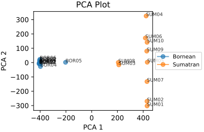
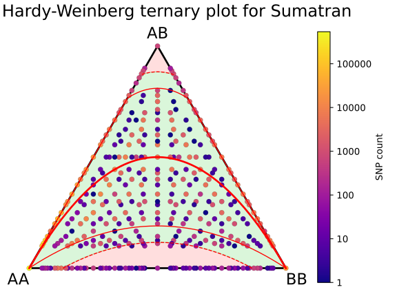
Popular Data Statistics
- Site frequency spectrum
Tools: dadi, fastsimcoal2 - Linkage Disequilibrium (LD)
Tools: momentsLD, GONE - Patterns of heterozygosity/homozygosity
Tools: PSMC, MSMC - IBD/IBS tracts
Tools: IBDNe
Site Frequency Spectrum
Site Frequency Spectrum
Derived allele is a new allele formed by mutation.
Site frequency spectrum (SFS) of P populations is the joint distribution of the derived allele frequencies of a given set of sites (SNP’s) across P populations.


Site Frequency Spectrum Example
| Reference: | ATACGTC | |
| 1 population | 2 population | |
| 1 individual | ATCCGAC | ACACTTC |
| 2 individual | ACACGTC | ACACGTT |
| 3 individual | GCACGTC |
| Position | 1 | 2 | 3 | 4 | 5 | 6 | 7 |
| Der. allele | G | C | C | - | T | A | T |
| Freq. in 1 pop. | 1 | 2 | 1 | - | 0 | 1 | 0 |
| Freq. in 2 pop. | 0 | 2 | 0 | - | 1 | 0 | 1 |


$$
A =
\begin{matrix}
\scriptsize 3 \\
\scriptsize 2 \\
\scriptsize 1 \\
\scriptsize 0 \\
\\
\end{matrix}
\begin{matrix}
\begin{pmatrix}
0 & 0 & 0 \\
0 & 0 & 0 \\
0 & 0 & 0 \\
0 & 0 & 0
\end{pmatrix} \\
\begin{matrix}
\scriptsize 0 & \scriptsize 1 & \scriptsize 2
\end{matrix} \\
\end{matrix}
$$
$$
A =
\begin{matrix}
\scriptsize 3 \\
\scriptsize 2 \\
\scriptsize \htmlData{class=fragment highlight-current-blue, fragment-index=3}{1} \\
\scriptsize 0 \\
\\
\end{matrix}
\begin{matrix}
\begin{pmatrix}
0 & 0 & 0 \\
0 & 0 & 0 \\
1 & 0 & 0 \\
0 & 0 & 0
\end{pmatrix} \\
\begin{matrix}
\scriptsize \htmlData{class=fragment highlight-current-blue, fragment-index=3}{0} & \scriptsize 1 & \scriptsize 2
\end{matrix} \\
\end{matrix}
$$
$$
A =
\begin{matrix}
\scriptsize 3 \\
\scriptsize \htmlData{class=fragment highlight-current-blue, fragment-index=4}{2} \\
\scriptsize 1 \\
\scriptsize 0 \\
\\
\end{matrix}
\begin{matrix}
\begin{pmatrix}
0 & 0 & 0 \\
0 & 0 & 1 \\
1 & 0 & 0 \\
0 & 0 & 0
\end{pmatrix} \\
\begin{matrix}
\scriptsize 0 & \scriptsize 1 & \scriptsize \htmlData{class=fragment highlight-current-blue, fragment-index=4}{2}
\end{matrix} \\
\end{matrix}
$$
$$
A =
\begin{matrix}
\scriptsize 3 \\
\scriptsize 2 \\
\scriptsize \htmlData{class=fragment highlight-current-blue, fragment-index=5}{1} \\
\scriptsize 0 \\
\\
\end{matrix}
\begin{matrix}
\begin{pmatrix}
0 & 0 & 0 \\
0 & 0 & 1 \\
2 & 0 & 0 \\
0 & 0 & 0
\end{pmatrix} \\
\begin{matrix}
\scriptsize \htmlData{class=fragment highlight-current-blue, fragment-index=5}{0} & \scriptsize 1 & \scriptsize 2
\end{matrix} \\
\end{matrix}
$$
$$
A =
\begin{matrix}
\scriptsize 3 \\
\scriptsize 2 \\
\scriptsize 1 \\
\scriptsize \htmlData{class=fragment highlight-current-blue, fragment-index=7}{0} \\
\\
\end{matrix}
\begin{matrix}
\begin{pmatrix}
0 & 0 & 0 \\
0 & 0 & 1 \\
2 & 0 & 0 \\
0 & 1 & 0
\end{pmatrix} \\
\begin{matrix}
\scriptsize 0 & \scriptsize \htmlData{class=fragment highlight-current-blue, fragment-index=7}{1} & \scriptsize 2
\end{matrix} \\
\end{matrix}
$$
$$
A =
\begin{matrix}
\scriptsize 3 \\
\scriptsize 2 \\
\scriptsize \htmlData{class=fragment highlight-current-blue, fragment-index=8}{1} \\
\scriptsize 0 \\
\\
\end{matrix}
\begin{matrix}
\begin{pmatrix}
0 & 0 & 0 \\
0 & 0 & 1 \\
3 & 0 & 0 \\
0 & 1 & 0
\end{pmatrix} \\
\begin{matrix}
\scriptsize \htmlData{class=fragment highlight-current-blue, fragment-index=8}{0} & \scriptsize 1 & \scriptsize 2
\end{matrix} \\
\end{matrix}
$$
$$
A =
\begin{matrix}
\scriptsize 3 \\
\scriptsize 2 \\
\scriptsize 1 \\
\scriptsize \htmlData{class=fragment highlight-current-blue, fragment-index=9}{0} \\
\\
\end{matrix}
\begin{matrix}
\begin{pmatrix}
0 & 0 & 0 \\
0 & 0 & 1 \\
3 & 0 & 0 \\
0 & 2 & 0
\end{pmatrix} \\
\begin{matrix}
\scriptsize 0 & \scriptsize \htmlData{class=fragment highlight-current-blue, fragment-index=9}{1} & \scriptsize 2
\end{matrix} \\
\end{matrix}
$$
Site Frequency Spectrum
Site Frequency Spectrum
Site Frequency Spectrum
Site Frequency Spectrum
Demographic Inference Tools
Demographic Inference Tools
: Model-free
PSMC

Source: Cousins et al. (2025)
GONE

Source: Santiago et al. (2020)
Demographic Inference Tools
: Model-based


Demographic Inference Tools
: Model-based
Examples:
- $\partial a \partial i$ [Gutenkunst et al. 2009]
- moments [Jouganous et al. 2017]
- momentsLD [Ragsdale and Gravel 2019, 2020]
- momi2 [Kamm et al. 2020]
- fastsimcoal2 [Excoffier et al. 2013, 2021]
- Dical2 [Steinrücken et al. 2019]
Issues of Existing Tools
Issue 1: Model Specification


Specification
for $\partial a \partial i$
Issue 2: Model Selection


Issue 3: Optimization

Most tools use local search optimization algorithms:
- BFGS
- Nelder–Mead method
- Powell's method
- EM, ECM
They require initial estimation and perform search for local optimum.
Local vs Global Optimization



GADMA — Global search Algorithm for Demographic Model Analysis
- Several likelihood engines ($\partial a \partial i$, moments, momi2, momentsLD)
- Common interface
- New model specification
- Effective global optimization

[Noskova et al. 2020] [Noskova et al. 2023]
New Model Specification
New Model Specification
New model in GADMA that is specified only by the number of epochs.


Available up to three populations
Flexible Dynamics
New model in GADMA has flexible dynamics of population size change.
Population dynamic can be:
- Constant (sudden change)
- Linear
- Exponential


Additional controls


Global Optimization:
Genetic Algorithm
Global Optimization:
Genetic Algorithm
Genetic algorithm:
- Widely used global optimization.
- Uses ideas of evolution and natural selection.
- Can discover solutions in large search space.
GADMA implements a combination of the genetic algorithm followed by a local search method.
Hyperparameters of the genetic algorithm are optimized (SMAC).
Demographic Inference
for Four and Five Populations
Demographic Inference
for Four and Five Populations
Challenges:
- Time-expensive likelihood evaluations
- Many phylogenetic tree topologies
- Great number of model parameters

GADMA:
Bayesian Optimization
Bayesian Optimization
Machine learning-based technique for optimizing expensive functions.
Enables demographic inference for 4 and 5 populations in GADMA.
[Noskova and Borovitskiy, 2023] [Example run]
Usecase 1:
Human Out-Of-Africa History
Human Out-Of-Africa History


History obtained by GADMA has better likelihood and CLAIC.
Usecase 2:
Using Different Likelihood Engines
Stdpopsim
: Easy Data Simulation


Likelihood Engines Comparison

$\partial a \partial i$


moments


momi2


momentsLD


Ground truth: 2,200
Usecase 3:
Four Population Demographic Inference
Four Population Demographic Inference


History obtained by GADMA has better likelihood.
Thank you!

Slides:
Starting Tutorial
You can view all the materials online:
You can download the repository to your local system (optional):
- git clone --depth 1 https://github.com/noscode/GADMA_workshops.git
- To update: git pull
- Materials are located in:
GADMA_workshops/2025-12-Demographic_Inference_Worshop/tutorials
Remember to activate your conda environment:
- $ conda activate gadma_workshop_env
Starting Tutorial
- Log in to the cluster and open bash interface
- Create a working directory:
mkdir your_name - Go to your working directory:
cd your_name - Copy the data:
cp -r ../Ekaterina_workshop/GADMA_workshop . - Copy the easySFS folder:
cp -r ../software/easySFS . - Activate computational node (srun command)
- Run:
conda activate gadma_workshop_env
EasySFS Tutoral
GADMA Tutoral
Model Selection Tutoral
Go to the directory: 3_Model_Selection_tutorial
Notebook: 3_Model_Selection_tutorial.ipynb